Getting Started
First Step in OpenFoam
Once you have installed OpenFOAM, hopefully without losing your mind, you can start its environment by typing in the terminal
openfoamXXXX
where XXXX is the version selected during the download.
From now on, the journey begins.
Your First Case:
To run your first simulation, it is essential to understand how the software operates. Each simulation is organized into several sub-folders:
- "Simulation_1"
- "0"
- "constant"
- "system"
The 0 directory contains specifications for the boundary fields, including patch type and initial values.
The constant directory houses the geometry, mesh and files that define constant values, such as fluid or turbulence properties.
The system directory hold all the instruction needed, including the Solver, numeric schemes, number of iterations, multi-processing options, and more.
This is a brief overview of how a general case is structured in OpenFOAM. Below an illustration of how the directory should look. To clarify the upcoming paragraphs, we will use a tutorial located in the OpenFOAM sub-directory. You can access it by typing the following commands in your terminal :
cd $FOAM_TUTORIALS
cd incompressible/simpleFoam/motorBike/
0 directory

The 0 directory contain the following files :
- "0.orig"
- U
- p
- nut
- k
- omega
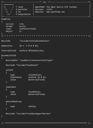
There is also another directory "include", but for now ignore it. The image on the right show how the file is structured.
In particular the image is referred to the U file, but all of them have the same structure. The file is like a key-value dictionary where the first key encountered is dimension, following internalField and boundaryField (we skipped the "#include" for now) . The dimension, as we can imagine, define the physical dimensional unit of the field. The array [ ... ] has 7 slots that represent 7 different units in this order:
| No. | Property | SI unit | USCS unit |
| 1 | Mass | kilogram (kg) | pound-mass (lbm) |
| 2 | Length | metre (m) | foot (ft) |
| 3 | Time | second (s) | second (s) |
| 4 | Temperature | Kelvin (K) | degree Rankine (R) |
| 5 | Quantity | mole (mol) | mole (mol) |
| 6 | Current | ampere (A) | ampere (A) |
| 7 | Luminous intensity | candela (cd) | candela (cd) |
The number given to the array represent the order of the dimension, for example is [0 1 -1 0 0 0 0].
Internal field key represent the value of the field at the beginning.
The boundary field key contains all the boundary conditions defined in the mesh. Each of them need a type and the relative options. Here is linked the standard boundary conditions list for OpenFOAM.
The # include command simply copy and past the given file's content. So in the "Include/initialConditions", for example, we wrote all initial conditions for the case, like velocity, pressure ecc... and then import it into U file. The internalField key set the field value, the $ symbol get the associated value.
Constant Directory

The constant directory contain the following files :
- "constant"
- transportProperties
- turbulenceProperties
- ObjectFile - "polyMesh"
The last element in the list simply represent a 3D object or an already meshed object for OpenFOAM, underling that we need a specific mesh file/files for this software.
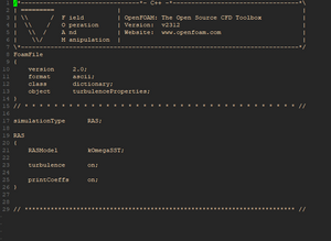
The other two file, transportProperties and turbulenceProperties , contains respectively the fluid physic properties, such dynamic viscosity or in general transport constant, and the turbulence model. On the left are showed images for both files.
In this example the turbulenceProperties file is set with a RAS (Reynolds Averaged Simulation) and the model selected is kOmegaSST. Values of k and omega are setted in the 0 directory, in the same name files.
System directory

The system directory can contain many files. In particular, you can create your own script in C++ using the OpenFOAM library to achieve complete customization. The main files of interest are:

- "system"
While there are additional files needed to create the mesh or collect information about the solution, exploring these files is not the focus of this page.
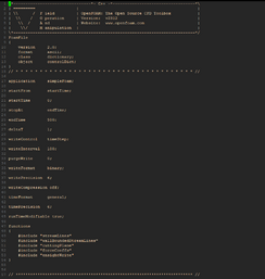
The controlDict is the core of the simulation. It specifies the simulation method ,here simpleFoam is the SIMPLE method, along with other important details such as the iteration number, start and end times of the simulation, and more. The function key allow the user to add existing function, like forceCoeffs , to evaluate aerodynamics coefficients in a specific reference system.
fvSchemes and fvSolution contains the divergence schemes for all the fields, gradients, flux, etc., as well as the solvers for each field, complete with various controls on residuals, tolerances, and other parameters. We will not delve deeply into these two files, as they are quite complex and not the focus of this section.
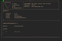
Lastly, the decomposePar, allow the user to decompose the case in different part using various methods. In this example the hierarchical method is employed, specifying how many pieces the case should be split into. This decomposition aims to parallelize the process across CPU cores, thereby speeding up the solution.
Run your case :
We are finally ready to start the simulation. In the case directory, you will find two files named Allrun and Allclean. These are bash scripts that enable the user to clean up the case and initiate the simulation by typing:
/Allclean
/Allrun
If these file are not executable, run the following command:
/chmod +x /All*
However, it's beneficial to learn how to perform these actions manually:
cp ./0.orig ./0
decomposePar
mpirun -np "N" "methodName" -parallel
cp ./0.orig ./0 simply copy the 0.orig directory in the same path and rename it in 0. That is necessary because OpenFOAM search 0 and not 0.orig.
decomposePar start the decomposition of the case, splitting the mesh and apply boundaries, in order to parallelize the process.
mpirun -np "N" "methodName" -parallel
The above command run the case in parallel. N are your core numbers, methodName is the method selected in the controlDict file. In this example we are using simpleFoam. if mpi is not installed it is possible to get it with the following commands
sudo update
sudo apt-get install openmpi
Now you are finally running your first simulation in OpenFOAM!
Post processing
When the simulation end, we are ready to give a look. On the console run this command:
reconstrucPar -latestTime
This recompose your last iteration from processor directories. Last command needed it
paraFoam
This will load mesh and result in paraview. If it is not installed on your device, it is possible to obtain with
sudo update
sudo apt install paraview